翻译国外文章,该文章介绍了Android开发中矩阵相关的数学知识,包括矩阵是什么?矩阵加法及乘法运算,2x2矩阵的变换,最后演进为Android中使用的3x3矩阵。文中图片及动图比较多,相对好懂。
原文链接:https://i-rant.arnaudbos.com/matrices-for-developers/#technical-challenge
几周前,我在一个android-user-group频道上,有人问一个关于Android的Matrix.postScale(sx,sy,px,py)方法及其工作原理的问题,因为它“难以掌握”。
在2016年初,我在一个Android应用程序上完成了一个自由项目,在其中我必须实现一个令人兴奋的功能:
用户在购买并下载了岩壁的数字地形后,必须能够查看由以下部分组成的岩壁:
- 悬崖的照片,
- 包含爬坡路线叠加层的SVG文件。
用户必须具有随意平移和缩放的能力,并且必须具有“跟随”图片的路线层。
| APP截图1 | APP截图2 | APP截图3 |
|---|---|---|
 |  |  |
技术挑战
为了让攀爬路线的图层能够跟随用户的手势操作,我发现我不得不重载Android ImageView,在Canvas上绘制并处理手指手势。 作为一名优秀的工程师:我搜索了Stack Overflow😅 我发现需要android.graphics.Matrix类进行2D转换。
这个类的问题在于,从方法名称来说,你能很清楚的了解它的作用,但是如果没有没有一定的数学背景知识,你很难了解它背后是怎么实现的,比方说下面是matrix的某个方法的API文档说明:
boolean postScale (float sx, float sy, float px, float py)
Postconcats the matrix with the specified scale. M’ = S(sx, sy, px, py) * M
从文档看起它可以通过某些参数缩放某些东西,并通过某种乘法来完成它。不过我还是有很多疑问:
- 它到底是做什么的? 缩放矩阵? 那是什么意思,我想缩放画布…
- 我应该使用preScale还是postScale? 当我从从手势检测代码获取输入参数,然后进入尝试和错误的无限循环时,是否需要尝试同时使用这两个方法?
因此,在开发过程的这一刻,我意识到在完成大学的头两年后,我需要重新学习很多年前关于矩阵的基本数学技能。
在搜寻网络资料时,我发现了很多不错的资源,并且能够再次学习一些数学知识。 通过将我的理解应用到Java和Android中的代码,它还帮助我解决了2D转换问题。 因此,考虑到我在上面提到的频道上进行的讨论,似乎我不是唯一一个在矩阵中苦苦挣扎的人,试图弄明白这一点,并在Android的Matrix类和方法中使用这些技能,所以我想我会写一篇文章,第一部分是关于矩阵的,第二部分“使用Android和Java进行2D转换”是关于如何在Java和Android上将关于矩阵的知识应用到代码中。
Matrix是什么?
我在可汗学院(Khan Academy)上发现一门关于矩阵的很好的代数课程。
如果你也遇到此类问题,我觉得你也可以花时间来学习这个课程,等到你觉得“原来就是这样”,就差不多了。实际上学习这些课程只需几个小时的投资,而且课程是免费的,你一定不会后悔。
矩阵擅长表示数据,所以对矩阵的操作可以帮助您解决此数据上的问题。还记得在学校必须解线性方程组吗?
解线性方程组最常见方法(至少是我研究过的两种方法)是消元法或行减少方法。不过,我们也可以使用矩阵来进行线性方程组的求解。
矩阵在每个科学分支中都大量使用,它们也可以用于线性变换来描述点在空间中的位置,这就是我们将在本文中简要研究的。
解刨
简单来说,矩阵是一个二维数组,实际上,一个 $m\ \times n$ 的矩阵可以对应于一个长度为 $m$ 的数组,该数组的每个item是另外一个长度为 $n$ 的数组。 通常来说 $m$ 代表了行数,$n$ 代表列数,matrix中的每个元素称之为 条目-$entry$ .
矩阵使用一个粗体大写字母表示,每个 $entry$ 使用对应的小写字母表示,同时使用行号和列号组合成为下标,一个矩阵的示例如下: $$ \textbf{A} = \begin{pmatrix} a_{11} & a_{12} & … & a_{1n} \ a_{21} & a_{12} & … & a_{1n} \ ⋮ & ⋮ & ⋱ & ⋮ \ a_{m1} & a_{m2} & … & a_{mn} \ \end{pmatrix} $$
接下来我们将学习矩阵的一些运算:加法和减法和乘法(multiplication)。
加法和减法
矩阵的加法和减法是通过矩阵的相应的entry相加或相减来完成的,计算方式如下: $$ \textbf{A} + \textbf{B} = \begin{pmatrix} a_{11} & a_{12} & … & a_{1n} \ a_{21} & a_{12} & … & a_{1n} \ ⋮ & ⋮ & ⋱ & ⋮ \ a_{m1} & a_{m2} & … & a_{mn} \ \end{pmatrix} + \begin{pmatrix} b_{11} & b_{12} & … & b_{1n} \ b_{21} & b_{12} & … & b_{1n} \ ⋮ & ⋮ & ⋱ & ⋮ \ b_{m1} & b_{m2} & … & b_{mn} \ \end{pmatrix}= \begin{pmatrix} a_{11} + b_{11} & a_{12}+b_{12} & … & a_{1n}+b_{1n} \ a_{21}+b_{21} & a_{12}+b_{12} & … & a_{1n}+b_{1n} \ ⋮ & ⋮ & ⋱ & ⋮ \ a_{m1}+b_{m1} & a_{m2}+b_{m2} & … & a_{mn}+b_{mn} \ \end{pmatrix} $$ 从上面的计算方式可以确定,矩阵的加法和减法只能是两个具有相同维度($m \times n$)的矩阵之间进行;
加法示例: $$ \textbf{A} + \textbf{B} = \begin{pmatrix} 4 & -8 & 7 \ 0 & 2 & 3 \ 15 & 4 & 9 \ \end{pmatrix} + \begin{pmatrix} -5 & 2 & 3 \ 4 & -1 & 6 \ 0 & 12 & 3 \ \end{pmatrix}= \begin{pmatrix} 4+(-5) & (-8)+2 & 7+3 \ 0+4 & 2+(-1) & (-1)+6 \ 15+0 & 4+12 & 9+3 \ \end{pmatrix}= \begin{pmatrix} -1 & -6 & 10 \ 4 & 1 & -5 \ 15 & 16 & 12 \ \end{pmatrix} $$
减法示例: $$ \textbf{A} + \textbf{B} = \begin{pmatrix} 4 & -8 & 7 \ 0 & 2 & 3 \ 15 & 4 & 9 \ \end{pmatrix}+ \begin{pmatrix} -5 & 2 & 3 \ 4 & -1 & 6 \ 0 & 12 & 3 \ \end{pmatrix}= \begin{pmatrix} 4-(-5) & (-8)-2 & 7-3 \ 0-4 & 2-(-1) & (-1)-6 \ 15-0 & 4-12 & 9-3 \ \end{pmatrix}= \begin{pmatrix} 9 & -10 & 4 \ -4 & 3 & -7 \ 15 & -8 & 6 \ \end{pmatrix} $$
矩阵乘法
上数学课的时候,老师说过:“你不能在橘子里加苹果,这是没有道理的”,然后告诉我们单位在运算中的重要性,也就是不同单位的操作数不能进行运算。
但是,对于矩阵来说,苹果和橙子相乘是合法的,我们只能将矩阵加到相同维度的矩阵上,但是我们可以将矩阵与数字和其他维度不同的矩阵相乘。
标量 $\times$ 矩阵
在矩阵的乘法中,单一的数字实际上应该称之为标量($\textbf{scalar}$),下面的运算中,实际上不是将矩阵乘以数字,而是将矩阵乘以标量。矩阵乘以标量的计算方式是:将矩阵中的每个条目乘以标量,然后得到另外一个矩阵。
$$
\textit{k} . \textbf{A} =
\textit{k} .
\begin{pmatrix}
a_{11} & a_{12} & … & a_{1n} \
a_{21} & a_{12} & … & a_{1n} \
⋮ & ⋮ & ⋱ & ⋮ \
a_{m1} & a_{m2} & … & a_{mn} \
\end{pmatrix}=
\begin{pmatrix}
\textit{k} . a_{11} & \textit{k} . a_{12} & … & \textit{k} . a_{1n} \
\textit{k} .a_{21} & \textit{k} . a_{12} & … & \textit{k} . a_{1n} \
⋮ & ⋮ & ⋱ & ⋮ \
\textit{k} .a_{m1} & \textit{k} . a_{m2} & … & \textit{k} . a_{mn} \
\end{pmatrix}
$$
一个简单的示例如下:
$$
4 . \begin{pmatrix}
0 & 3 & 12 \
7 & -5 & 1 \
-8 & 2 & 0 \
\end{pmatrix} =
\begin{pmatrix}
0 & 12 & 48 \
28 & -20 & 4 \
-32 & 8 & 0 \
\end{pmatrix}
$$
矩阵 $\times$ 矩阵
另外一种矩阵乘法就是 矩阵乘以矩阵 ,矩阵乘法运算起来稍微有点复杂,因为我们并不能简单的对应的entry进行乘法运算,具体计算规则我们直接看维基百科的说明:
如果 $\mathbf{A}$ 是一个 $m \times n$ 的 矩阵,$\mathbf{B}$ 是一个 $n \times p$ 的matrix, 那么它们的矩阵乘积 $\mathbf{AB}$ 是一个 $m \times p $的矩阵,
其中矩阵 $\mathbf{A}$ 行中的 $n$ 个条目与矩阵 $\mathbf{B}$ 列中的 $n$ 个条目 相乘并求和 得出矩阵 $\mathbf{AB}$ 的条目。
看起来有点复杂,让我们逐段分解的来看:
如果 $\mathbf{A}$ 是一个 $m \times n$ 的 矩阵,$\mathbf{B}$ 是一个 $n \times p$ 的matrix, 那么它们的矩阵乘积 $\mathbf{AB}$ 是一个 $m \times p$ 的矩阵
上面的规则我们可以写成: $\mathbf{A}{m \times n} \times \mathbf{B}{n \times p} = \mathbf{AB}_{m \times p}$
看一个简单的矩阵 $\mathbf{A}{2 \times 3} = \begin{pmatrix} a{11} & a_{12} & a_{13} \ a_{21}&a_{22}&a_{23} \end{pmatrix}$ 和另外一个矩阵 $\mathbf{B}{3 \times 1} = \begin{pmatrix} b{11} \ b_{21} \ b_{31} \end{pmatrix}$ ,这里$m = 2, n=3, p=1$,所以矩阵乘积为一个$2\times1$的矩阵: $\mathbf{AB}=\begin{pmatrix} ab_{11} \ ab_{12} \end{pmatrix}$。
接下来我们分解第二部分:
- ==矩阵 $\mathbf{A}$ 行中的 $n$ 个条目== 指的是:矩阵 $\mathbf{A}$ 的每一行都是一个 $n=3$ 的数组,第一行我们可以记为 $a_{11}, a_{12} , a_{13}$
- ==矩阵 $\mathbf{B}$ 列中的 $n$ 个条目== 指的是:矩阵 $\mathbf{B}$ 中的每一列也是一个 $n=3$ 的数组,第一列可以记为: $b_{11}, b_{12} , b_{13}$
- ==相乘== 指: $\mathbf{A}$ 的行中的每个条目都与 $\mathbf{B}$ 的列中的每个对应条目一一相乘(第一个条目对应第一个,第二对第二,依次),结果就是:$a_{11} \times b_{11}, a_{12} \times b_{12} \ 和 \ a_{13} \times b_{13}$
- ==求和== 指:累加这些对应的行和列条目的乘积,得到新的矩阵在该行号和列号处的新的条目,新的条目的值为:$a_ {11} \times b_ {11} + a_ {12} \times b_ {21} + a_{13} \times b_ {31}$
$$ \mathbf{A} = \begin{pmatrix} a_{11} & a_{12} & \cdots & a_{1n}\ a_{21} & a_{22} & \vdots & a_{2n}\ \vdots & \vdots & \ddots & \vdots\ a_{m1} & a_{m2} & \cdots & a_{mn} \end{pmatrix} \text{, } \mathbf{B} = \begin{pmatrix} b_{11} & b_{12} & \cdots & b_{1p}\ b_{21} & b_{22} & \vdots & b_{2p}\ \vdots & \vdots & \ddots & \vdots\ b_{n1} & b_{n2} & \cdots & b_{np} \end{pmatrix} \ \ \mathbf{AB} = \begin{pmatrix} ab_{11} & ab_{12} & \cdots & ab_{1p}\ ab_{21} & ab_{22} & \vdots & ab_{2p}\ \vdots & \vdots & \ddots & \vdots\ ab_{m1} & ab_{m2} & \cdots & ab_{mp} \end{pmatrix} \text{其中 } ab_{ij}=\sum_{k=1}^{m}a_{ik}b_{kj} $$
我们用一个可视化的方式来表示这个过程:

$$ \mathbf{A} = \begin{pmatrix} 4 & 3\ 0 & -5\ 2 & 1\ -6 & 8 \end{pmatrix} \text{, } \mathbf{B} = \begin{pmatrix} 7 & 1 & 3\ -2 & 4 & 1 \end{pmatrix} \ \begin{aligned} \mathbf{AB} &= \begin{pmatrix} 4\times7+3\times\left(-2\right) & 4\times1+3\times4 & 4\times3+3\times1\ 0\times7+\left(-5\right)\times\left(-2\right) & 0\times1+\left(-5\right)\times4 & 0\times3+\left(-5\right)\times1\ 2\times7+1\times\left(-2\right) & 2\times1+1\times4 & 2\times3+1\times1\ \left(-6\right)\times7+8\times\left(-2\right) & \left(-6\right)\times1+8\times4 & \left(-6\right)\times3+8\times1 \end{pmatrix}\\ &= \begin{pmatrix} 28-6 & 4+12 & 12+3\ 0+10 & 0-20 & 0-5\ 14-2 & 2+4 & 6+1\ -42-16 & -6+32 & -18+8 \end{pmatrix}\\ \mathbf{AB} &= \begin{pmatrix} 22 & 16 & 15\ 10 & -20 & -5\ 12 & 6 & 7\ -58 & 26 & -10 \end{pmatrix} \end{aligned} $$
注意:
为了定义矩阵乘法,==第一个矩阵中的列数==必须等于==第二个矩阵中的行数==。
了解更多:
变换矩阵
现在我们知道了矩阵是什么,并且知道矩阵如何相乘,接下来我们看下矩阵如何应用于二维变换;
转换点
正如之前所说,矩阵可以被用于表示线性方程组,假设我们有如下方程组: $$ 2x + y = 5 \ -x + 2y = 0 $$ 如果你对矩阵乘法很熟悉,你可能看到上述方程中隐藏的矩阵乘法: $$ \begin{pmatrix} 2 & 1 \ -1 & 2 \ \end{pmatrix} . \begin{pmatrix} x \ y \end{pmatrix}= \begin{pmatrix} 5 \ 0 \end{pmatrix} $$ 如果你看的更深一点,你可能会发现基于矩阵$\begin{pmatrix} x \ y \end{pmatrix}$ 和 $\begin{pmatrix} 5 \ 0 \end{pmatrix}$的一些规律。
那就是:这两个矩阵都可以被用来代表笛卡尔平面中的点,一个点可以用源自原点的向量表示,这个向量是一个 $2×1$ 的矩阵。
我们现在知道了一个矩阵乘法就代表了一个点到另外一个点的转换,尽管我们目前还不知道第一个点的坐标是什么,不过不用担心,我们只需要知道,给定一个位置矢量,我们就可以通过矩阵乘法运算将其转换为另外一个矢量。
如果一个点 $\mathbf{P}$ 是一个值为$\begin{pmatrix} x\y \end{pmatrix}$ 的位置矢量,我们可以乘一个矩阵来得到一个新的点 $\mathbf{P}^{’}$
它可以通过位置矢量 $\begin{pmatrix} x^{’} \ y^{’} \end{pmatrix}$ 来表示;
一个重要的点在于,为了满足矩阵乘法的要求,矩阵变换必须拥有特定的维度,因为源位置矢量 $\begin{pmatrix} x\y \end{pmatrix}$ 是一个 $2\times 1$ 的矩阵,而目标位置矢量 $\begin{pmatrix} x^{’} \ y^{’} \end{pmatrix}$ 也是一个 $2 \times 1$ 的矩阵,所以变换矩阵必须是一个 $2 \times 2$ 的矩阵,这样才能满足矩阵乘法的要求: $$ \mathbf{A} . \begin{pmatrix} x\y \end{pmatrix} = \begin{pmatrix} a_{11} & a_{12}\ a_{21} & a_{22} \end{pmatrix} . \begin{pmatrix} x\y \end{pmatrix} = \begin{pmatrix} x^{\prime}\y^{\prime} \end{pmatrix} $$
- 第一个矩阵的列数必须等于第二个矩阵的行数,所以第一个矩阵的列数需要为 2
- 矩阵相乘得到的矩阵的尺寸为 $第一个矩阵的行数 \times 第二个矩阵的列数$,为了得到一个 $2 \times 1$ 的结果矩阵,则==第一个矩阵的行数== 为 2
- 故变换矩阵的行列数为:$2 \times 2$
- 提示:后面我们会看到,矩阵乘法中的顺序很重要。比方说上面的矩阵乘法,如果调换 $\mathbf{A}$ 和 $\begin{pmatrix} x\y \end{pmatrix}$ 的顺序,则无法获得一个新的点: $P_{2\times1} . A_{1\times n}=P^{’}_{2 \times n}$(不成立)
转换矩阵的另外一个非常好用的地方在于,它可以同时批量的转换一批点;
$$ \mathbf{A} . \begin{pmatrix} x\y \end{pmatrix} = \begin{pmatrix} a_{11} & a_{12}\ a_{21} & a_{22} \end{pmatrix} . \begin{pmatrix} x\y \end{pmatrix} = \begin{pmatrix} x^{\prime}\y^{\prime} \end{pmatrix} $$
假设你知道所需要的应用的所有转换类型(rotation,scale,translation)及其他参数。
那么,如何获得缩放2倍并沿着顺时针方向旋转90度的转换矩阵呢?
答案是:我们需要更多数学知识。
更多数学知识
建议大家阅读此课程中有关变换的矩阵课程(其中有大量精美的图示和动画),特别是它的最后一部分:用矩阵表示二维线性变换,讲的非常不错;
回到我们刚才讨论的问题,现在让我们了解更多数学知识吧。
现在我假设你学习了上面的课程,下面的部分是对该课程的简单回顾:
一个位置矢量 $\begin{pmatrix}x \ y \end{pmatrix}$ 可以被表示为 : $\begin{pmatrix}x \ y \end{pmatrix} = x . \begin{pmatrix} \color{Green}1 \ \color{Green}0 \end{pmatrix} + y . \begin{pmatrix} \color{Red}0 \ \color{Red}1 \end{pmatrix}$
解释:
$\begin{pmatrix}x \ y \end{pmatrix}$ 可以被分解为一个矩阵加法运算: $\begin{pmatrix}x \ y \end{pmatrix} = \begin{pmatrix}x \ 0 \end{pmatrix} + \begin{pmatrix}0 \ y \end{pmatrix}$
其中的每个加法的运算矩阵都可以被继续拆分为一个标量同矩阵的乘法:
- $\begin{pmatrix} x \ 0 \end{pmatrix} = x . \begin{pmatrix} 1 \ 0 \end{pmatrix}$
- $\begin{pmatrix} 0 \ y \end{pmatrix} = y . \begin{pmatrix} 0 \ 1 \end{pmatrix}$
现在,我们看其中的矩阵 $\begin{pmatrix} 1\0 \end{pmatrix}$ 和 $\begin{pmatrix} 0 \1 \end{pmatrix}$,其实它们是笛卡尔坐标平面的单位矢量;
因此, $\begin{pmatrix}x \ y \end{pmatrix} = x . \begin{pmatrix} \color{Green}1 \ \color{Green}0 \end{pmatrix} + y . \begin{pmatrix} \color{Red}0 \ \color{Red}1 \end{pmatrix}$ 就是位置矢量 $\begin{pmatrix}x \ y \end{pmatrix}$ 的另外一种写法,它代表了由我们的笛卡尔平面的单位向量的变换给出的点。
在应用了变换矩阵$\mathbf{A} = \begin{pmatrix} \color{Green} a & \color{Red} b\ \color{Green} c & \color{Red} d \end{pmatrix}$ 之后, $\begin{pmatrix} \color{Green}a\\color{Green}c \end{pmatrix}$ 和 $\begin{pmatrix}\color{Red} b\ \color{Red} d\end{pmatrix}$ 将被分别放置于 $\begin{pmatrix} \color{Green}1 \ \color{Green}0 \end{pmatrix}$ 和 $\begin{pmatrix} \color{Red}0 \ \color{Red}1 \end{pmatrix}$ 的位置;
解释:
我们依然从单位矢量 $\begin{pmatrix} \color{Green}1 \ \color{Green}0 \end{pmatrix}$和 $\begin{pmatrix} \color{Red}0 \ \color{Red}1 \end{pmatrix}$ 开始
我们知道 $\begin{pmatrix}x \ y \end{pmatrix} = x . \begin{pmatrix} \color{Green}1 \ \color{Green}0 \end{pmatrix} + y . \begin{pmatrix} \color{Red}0 \ \color{Red}1 \end{pmatrix}$,现在我们想像一下,如果我们应用一个变换到我们的平面上,那么我们的单位矢量也会随之变换吧?
我们假设变换后 $\begin{pmatrix} \color{Green}1 \ \color{Green}0 \end{pmatrix}$ 会坐落在 $\begin{pmatrix} \color{Green}a \ \color{Green}c \end{pmatrix}$ 上,而$\begin{pmatrix} \color{Red}0 \ \color{Red}1 \end{pmatrix}$ 会落在 $\begin{pmatrix} \color{Red}b \ \color{Red}d \end{pmatrix}$ 上,那么我们的位置矢量 $\begin{pmatrix}x \ y \end{pmatrix}$ 将会落在 $x.\begin{pmatrix}\color{Green} a \ c \end{pmatrix} + y.\begin{pmatrix} \color{Red} b\d \end{pmatrix} = \begin{pmatrix}\color{Green}a.x + \color{Red}b.y \ {\color{Green}c.x + \color{Red}d.y} \end{pmatrix}$
经过上面的矩阵变换,$\begin{pmatrix} x \ y \end{pmatrix}$ 将会坐落于 $\begin{pmatrix} \color{Green}a.x + \color{Red}b.y \ \color{Green}c.x + \color{Red}d.y \ \end{pmatrix}$
如果你无法理解上面的变换过程,请学习上面的课程并反复阅读。
现在,我们需要明确我们的目标,就是:我们需要找出我们的变换矩阵 $\mathbf{A}$ ,因为我们知道了我们想要应用的转换,但是我们需要找到那个能够应用到我们的位置矢量上来转换我们图形的矩阵;
让我们以一系列点的转换为例:我们知道位置矢量将到达的位置,但是我们需要求出矩阵 $\mathbf{A}$ 。
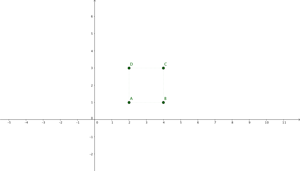
我们的笛卡尔平面上有一个由三个点 $\mathbf{P}{(2,1)},\mathbf{Q}{(2,0)} \mathbf{R}{(0,2)}$ P组成的三角形, 以及另一个代表第一个三角形的变换版本的三角形:$\mathbf{P}^{’}{(5,0)},\mathbf{Q}^{’}{(-4,2)} \mathbf{R}^{’}{(2,4)}$

上面的例子中我们只需要两个点就可以求解出矩阵$\mathbf{A}$,我们使用 $\mathbf{P}$ 和 $\mathbf{Q}$,我们知道,变换之后: $$ \begin{pmatrix} 2\ 1 \end{pmatrix} \text{ 位于 } \begin{pmatrix} 5\ 0 \end{pmatrix} \ \ \begin{pmatrix} -2\ 0 \end{pmatrix} \text{ 位于 } \begin{pmatrix} -4\ 2 \end{pmatrix} $$ 也就是说: $$ \begin{pmatrix} x\ y \end{pmatrix} = \begin{pmatrix} 2\ 1 \end{pmatrix} \text{ 位于 } \begin{pmatrix} a.x+b.y\ c.x+d.y \end{pmatrix} = \begin{pmatrix} 5\ 0 \end{pmatrix} \ \ \begin{pmatrix} x\ y \end{pmatrix} = \begin{pmatrix} -2\ 0 \end{pmatrix} \text{ 位于 } \begin{pmatrix} a.x+b.y\ c.x+d.y \end{pmatrix} = \begin{pmatrix} -4\ 2 \end{pmatrix} $$ 简化之后就是: $$ \begin{pmatrix} 2.a+1.b\ 2.c+1.d \end{pmatrix} = \begin{pmatrix} 5\ 0 \end{pmatrix} \ \begin{pmatrix} -2.a+0.b\ -2.c+0.d \end{pmatrix} = \begin{pmatrix} -4\ 2 \end{pmatrix} $$ 通过第2个等式可以算出, $a=2$ ,$c=-1$,代入到第一个等式中可以得出: $b=1$, $d =2$,现在我们得到了我们的变换矩阵: $$ \mathbf{A} = \begin{pmatrix} \color{Green} 2 & \color{Red} 1\ \color{Green} -\color{Green} 1 & \color{Red} 2 \end{pmatrix} $$
单位矩阵
现在我们还不知道如何定义一个转换矩阵,但是我们知道它的表示形式。接下来我们要做什么呢?还记得在上一个小节中,我们说过,一个位置$\begin{pmatrix}x \ y \end{pmatrix}$ 可以被表示为 $\begin{pmatrix}x \ y \end{pmatrix} = x . \begin{pmatrix} \color{Green}1 \ \color{Green}0 \end{pmatrix} + y . \begin{pmatrix} \color{Red}0 \ \color{Red}1 \end{pmatrix}$ ,这是一个很好的起点,我们刚刚列出了我们的==基本==矩阵:
$$ \begin{pmatrix} \color{Green}1 & \color{Red}0 \ \color{Green} 0 & \color{Red} 1 \end{pmatrix} $$
这个矩阵代表了你的平面的基础状态,也就是刚加载图像时应用于平面的矩阵(图像与其变换后的容器视图的大小相同),换一种说法就是,应用了这个矩阵的位置矢量将会返回一样的位置矢量。这样的矩阵就称之为 ==单位矩阵==(identity matrix)
结合多种变换
在我们了解更多细节之前,还有一件事,就是:我们希望用户能够组合/链接多种变换(例如,同时缩放和平移)。
为了能链接多个转换,我们需要理解矩阵乘法的性质 。更具体的说是我们需要了解矩阵乘法的==非交换性(non-commutative)==和==结合性==(associative)
- 矩阵乘法是可结合的: $\left(\mathbf{A}.\mathbf{B}\right).\mathbf{C} = \mathbf{A}.\left(\mathbf{B}.\mathbf{C}\right)$
- 矩阵乘法是不可交换的:$\mathbf{A}.\mathbf{B} \neq \mathbf{B}.\mathbf{A}$
回到我们的变换,想象我们想要应用变换 $\mathbf{B}$ ,然后应用变换 $\mathbf{A}$ 到我们的位置矢量 $\vec{v}$ ,两次变换可以分别表示为:$\vec{v^{\prime}} = \mathbf{B} . \vec{v}$ 及 $\vec{v^{\prime\prime}} = \mathbf{A} . \vec{v^{\prime}}$ ,结合下来:
$$ \vec{v^{\prime\prime}} = \mathbf{A} . \left( \mathbf{B} . \vec{v} \right) $$ 因为矩阵乘法是可以结合的,所以: $$ \vec{v^{\prime\prime}} = \mathbf{A} . \left( \mathbf{B} . \vec{v} \right) \Leftrightarrow \vec{v^{\prime\prime}} = \left( \mathbf{A} . \mathbf{B} \right) . \vec{v} $$ 因为矩阵乘法是不可交换的,所以两个变换矩阵的应用顺序不可改变,即 $\mathbf{A}.\mathbf{B}$ 不能变换成 $\mathbf{B}.\mathbf{A}$,否则将会产生不同的变换效果;
注意这里矩阵变换应用的顺序和转换成乘法之后的矩阵顺序,我们先应用$\mathbf{B}$,然后再应用 $\mathbf{A}$,结合之后的顺序是 :$\mathbf{A.B}$
变换类型
使用 $2\times2$ 的矩阵我们可以定义多种不同类型的二维变换类型,你可能已经在课程 matrices as transformations 中了解了其中的大部分变换,这些变换包括:
- 缩放
- Reflexion-反射
- Shearing
- Rotation-旋转
本小节中,我们假设我们有一个点 $\mathbf{P}{(x,y)}$,这个点代表了平面中的任一个点,我们希望找到一个矩阵能将点转换到 $\mathbf{P^{’}}{(x^{’},y^{’})}$,也就是: $$ \begin{pmatrix} x^{\prime}\y^{\prime} \end{pmatrix} = \mathbf{A} . \begin{pmatrix} x\y \end{pmatrix} = \begin{pmatrix} a & b\c & d \end{pmatrix} . \begin{pmatrix} x\y \end{pmatrix} $$
Scaling
缩放看起来很好表示,比方说放大2倍,只需将坐标乘以比例因子就可以了,但是我们可能希望对转换使用不同的水平和垂直缩放比例,这种情况下我们应该怎么做呢?
为了能够在不同的方向使用不同的缩放比例,我们必须区分水平和垂直方向的缩放比例,它们分别使用$S_{x}$ 和$S_{y}$表示;
我们可以得到如下两个等式: $$ \begin{aligned} x’ &= S_{x} . x \ y’ &= S_{y} . y \end{aligned} $$ 结合之前的矩阵: $$ \begin{pmatrix} x^{\prime}\y^{\prime} \end{pmatrix} = \begin{pmatrix} a & b\c & d \end{pmatrix} . \begin{pmatrix} x\y \end{pmatrix} $$ 我们可以得到 $a,b,c,d$ 如下: $$ \left. \begin{aligned} S_{x} . x &= a . x + b . y\\ \Rightarrow a &= S_{x} \text{ 且 }\ b &= 0 \end{aligned} \middle | \begin{aligned} S_{y} . y &= c . x + d . y\\ \Rightarrow c &= S_{y} \text{ 且 }\ d &= 0 \end{aligned} \right. $$
缩放比例$(S_x,S_y)$ 对应的 $2\times2$ 缩放矩阵就是: $$ \begin{pmatrix} a & b\c & d \end{pmatrix} = \begin{pmatrix} S_x & 0\0 & S_y \end{pmatrix} $$ 当缩放比例为 $1$ 时,应用这个缩放矩阵是: $$ \begin{pmatrix} S_{x} & 0\0 & S_{y} \end{pmatrix} = \begin{pmatrix} 1 & 0\0 & 1 \end{pmatrix} $$ 也就是单位矩阵,应用之后 $x$,$y$ 均不会改变,这与单位矩阵的意义符合。
Reflexion-仿射
仿射,我们可以考虑两种前方的仿射类型:围绕轴或围绕点的仿射。
为简单起见,我们将重点放在$x$和$y$轴周围的仿射(原点周围的反射等同于在$x$和$y$轴上连续施加仿射)。
围绕 $x$ 轴的反射: $$ \left.\begin{aligned} x^{\prime} &= x\ x &= a . x + b . y\\ \Rightarrow a &= 1 \text{ and }\ b &= 0 \end{aligned} \middle| \begin{aligned} y^{\prime} &= -y\ -y &= c . x + d . y\\ \Rightarrow c &= 0 \text{ and }\ d &= -1 \end{aligned} \right. $$ 有趣的是,围绕 $x$ 轴的仿射和使用 -1 作为缩放因子对$x$ 进行缩放的转换矩阵一致; $$ \begin{pmatrix} a & b\c & d \end{pmatrix} = \begin{pmatrix} 1 & 0\ 0 & -1 \end{pmatrix} $$ 围绕 $y$ 轴方向的仿射: $$ \left. \begin{aligned} x^{\prime} &= -x\ -x &= a . x + b . y\\ \Rightarrow a &= -1 \text{ and }\ b &= 0 \end{aligned} \middle| \begin{aligned} y^{\prime} &= y\ y &= c . x + d . y\\ \Rightarrow c &= 0 \text{ and }\ d &= 1 \end{aligned} \right. $$ 转换矩阵: $$ \begin{pmatrix} a & b\c & d \end{pmatrix} = \begin{pmatrix} -1 & 0\ 0 & 1 \end{pmatrix} $$
Shearing-剪切
这个Shearing变换有些复杂。
在我发现的大多数示例中,剪切都是通过添加一个可以代表shearing角度的常量来更改坐标来解释的。
比方说,一个沿着$x$ 轴方向的 shear 通常使用一个顶点位于$(0,1)$ 的矩形变换成一个顶点位于 $(1,1)$ 的平行四边形来解释;

不过在这篇文章中,我想用剪切角(轴被剪切的角度)来解释它。我们称之为 $\alpha$ (alpha)。


如果看上面的平面,我们可以看到新的横坐标 $x^{\prime}$ 等于$x$加/减去$y$轴,$y$轴的剪切形式以及矩形左上角顶点与平行四边形左上角顶点之间的线段所形成的三角形的相对边。 换句话说,$x ^{\prime}$ 等于 $x$ 加/减绿色三角形的另一侧
 |  |
|---|---|
 |  |
在直角三角形中:
- 斜边(==hypotenuse==)是最长的一面
- 对边(==opposite==)是与给定角度相反的那一侧
- 相邻边(==adjacent==)是给定角度的下一个
- $\mathbf{PP^{’}}$ 是对边,为了计算$x^{’}$ 到 $x$ 的距离,我们需要计算出对边的长度 ($k$);
- 邻边就是 $P^{’}$ 的坐标: $y$ ;
- 我们不知道斜边的长度
在三角函数(trigonometry)中: $$ \begin{aligned} \cos \left( \alpha \right) &= \frac{邻边}{斜边}\\ \sin \left( \alpha \right) &= \frac{对边}{斜边}\\ \tan \left( \alpha \right) &= \frac{对边}{邻边} \end{aligned} $$ 现在,我们知道了 $\alpha$ ,但我们不知道斜边的长度,所以我们不能使用 cosine 函数。
另一方面,我们知道邻边的长度(也就是$y$),我一我们可以使用 tangent 函数来求出对边的长度: $$ \begin{aligned}\tan \left( \alpha \right) &= \frac{对边}{邻边}\\对边 &= 邻边 \times \tan \left( \alpha \right)\end{aligned} $$ 我们可以开始求解我们的线性方程组来得出我们需要的矩阵: $$ x^{\prime} = x + k = x + y . \tan \left( \alpha \right) \ y^{\prime} = y $$ 当 $\alpha > 0$ 时,$tan(\alpha) < 0$,当 $α<0, \tan \left( \alpha \right) > 0$ ,两种情况下,通过 $x′= x+k=x+y.tan(α)$ 求解出来的可能为正也可能为负;$\alpha > 0$ 为逆时针的旋转/斜切角,当 $α<0$ 时,为顺时针方向的旋转/斜切角。 $$ \left. \begin{aligned} x^{\prime} &= x + y . \tan \left( \alpha \right) \ x + y . \tan \left( \alpha \right) &= a . x + b . y\\ \Rightarrow a &= 1 \text{ and }\ b &= \tan \left( \alpha \right) \end{aligned} \middle| \begin{aligned} y^{\prime} &= y\ y &= c . x + d . y\\ \Rightarrow c &= 0 \text{ and }\ d &= 1 \end{aligned} \right. $$
沿$x$方向剪切的变换矩阵为: $$ \begin{aligned} \begin{pmatrix} a & b\c & d \end{pmatrix} = \begin{pmatrix} 1 & \tan \alpha \ 0 & 1 \end{pmatrix} = \begin{pmatrix} 1 & k_{x}\ 0 & 1 \end{pmatrix}\\ {\text{其中 } k_{x} \text{ 是 shearing 常量}} \end{aligned} $$ 类似的,沿 $y$ 方向剪切的变换矩阵为: $$ \begin{aligned} \begin{pmatrix} a & b\c & d \end{pmatrix} = \begin{pmatrix} 1 & 0\ \tan \beta & 1 \end{pmatrix} = \begin{pmatrix} 1 & 0\ k_{y} & 1 \end{pmatrix}\\ \text{其中 } k_{y} \text{ 是 shearing 常量} \end{aligned} $$
Rotation
旋转就更加复杂了。
我们仔细看下下面 围绕原点旋转 $\theta$ (theta)角度 的例子:


注意,两个点 $\mathbf{P}$ 和 $\mathbf{P}^{’}$ 在它们自己的坐标平面中都有相同的坐标$(x,y)$,但是 $\mathbf{P}^{’}$ 在第一个没有被旋转的坐标系中有新的坐标: $\left({x^{’},y^{’}}\right)$ 。
那么,现在我们可以定义原始坐标点$(x,y)$ 到新的坐标点 $\left({x^{’},y^{’}}\right)$ 之间的关系了吗?
我们可以使用三角函数来帮助我们计算,在寻找对应的解法时,我发现了尼克·贝里(Nick Berry)的基于几何的解释和此视频。
老实说,我对这种解决方案不是100%满意,因为我不完全理解了它。 在重新阅读我写的内容之后,Hadrien(审阅者之一)和我发现我的解释有些不是那么完美。因此,如果您有兴趣,我会把它留在这里,但我建议您不要打扰,除非您非常好奇并且不要介意一些混乱。
现在,为了进行简单的解释清楚旋转的概念,我将采用 此位置向量落在映射到另外一个位置向量上 的路线。
假设你像下图一样在单位矢量上进行缩放:

基于三角函数的规则,我们可以看得到: $$ \left. \begin{pmatrix} 0\ 1 \end{pmatrix} \text{ lands on } \begin{pmatrix} \cos \theta \ \sin \theta \end{pmatrix} \middle| \begin{pmatrix} 1\ 0 \end{pmatrix} \text{ lands on } \begin{pmatrix} - \sin \theta \ \cos \theta \end{pmatrix} \right. $$ 也就是: $$ \begin{pmatrix} x\ y \end{pmatrix} = \begin{pmatrix} 1\ 0 \end{pmatrix} \text{ lands on } \begin{pmatrix} a.x+b.y\ c.x+d.y \end{pmatrix} = \begin{pmatrix} \cos \theta \ \sin \theta \end{pmatrix} $$
$$ \begin{pmatrix} x\ y \end{pmatrix} = \begin{pmatrix} 0\ 1 \end{pmatrix} \text{ lands on } \begin{pmatrix} a.x+b.y\ c.x+d.y \end{pmatrix} = \begin{pmatrix} - \sin \theta \ \cos \theta \end{pmatrix} $$
我们可以推断出: $$ \left. \begin{pmatrix} 1.a+0.b\ 1.c+0.d \end{pmatrix} = \begin{pmatrix} \cos \theta \ \sin \theta \end{pmatrix} \middle| \begin{pmatrix} 0.a+1.b\ 0.c+1.d \end{pmatrix} = \begin{pmatrix} - \sin \theta \ \cos \theta \end{pmatrix} \right. $$ 很明显可以得出: $a = \cos\left(\theta \right), b = - \sin \left( \theta \right), c = \sin \left( \theta \right) ,而\ d = \cos \left( \theta \right)$ ,我们可以得到我们的旋转矩阵: $$ \begin{pmatrix} a & b\c & d \end{pmatrix} = \begin{pmatrix} \cos \theta & -\sin \theta\ \sin \theta & \cos \theta \end{pmatrix} $$ 恭喜你!现在你已经知道了如何定义缩放,仿射,剪切和旋转的变换矩阵。 那么,还差什么呢?
3x3 变换矩阵
如果你看到了这里,经过上面的解释,你可能知道了上述的单个变换为什么会起作用,但是,我们的目标其实是理解这些仿射变换,然后在代码中应用它们。
仅仅知道单个变换的用法也是很有用的,因为现在我们知道了变换矩阵长什么样,并且知道如何在给定的几个位置矢量的情况下计算一个变换矩阵,了解这些就已经非常了不起了。
但是,有一个问题就是:我们能通过 $2\times2$ 的矩阵所做的操作太少了,你只能做一些我们之间见到过的变换:
- Scaling - 缩放
- Reflexion - 仿射
- Shearing - 剪切
- Rotation - 旋转
那么我们还需要什么? 答案是: 平移-translations
平移非常有用,比方说当用户触摸图像并移动手指时,图片需要能跟随用户的手势一起移动;平移可以被定义为两个矩阵的加法: $$ \begin{pmatrix} x^{’} \ y^{’} \end{pmatrix} = \begin{pmatrix} x \ y \end{pmatrix} + \begin{pmatrix} t_x \ t_y \end{pmatrix} $$ 不过,我们希望用户能够联合执行多种变换(如以一个不是原点的点为中心进行缩放),因此我们需要找到将平移表示为矩阵乘法的方式。
这里可能涉及到 [Homogeneous coordinates](https://en.wikipedia.org/wiki/Homogeneous_coordinates 的世界,不过你可以不用了解这些。
这里关联概念就是:
- 我们使用的平面笛卡尔坐标平面实际上只是三维坐标空间中众多平面中的一个,其 $z$ 坐标 为 1
- 对于三维空间的任意点 $(x,y,z)$ 来说,投影空间中穿过这个点和原点的线,同时也会穿过使用相同的缩放比例对 $x,y,z$ 进行缩放后的点;
- 这条线上的任意点的坐标可以表示为:$\left(\frac{x}{z}, \frac{y}{z}, z\right)$

我在本文的末尾附上了我收集的相关文章及博客的链接,如果你感兴趣,可以继续深入阅读。
我们现在不仅可以将笛卡尔坐标系($z=1$)中的点表示为一个 $2\times1$ 的矩阵,也可以表示为一个 $3\times1$的矩阵: $$ \begin{pmatrix} x\ y \end{pmatrix} \Leftrightarrow \begin{pmatrix} x\ y\ 1 \end{pmatrix} $$ 不过这也意味着我们需要重新定义我们之前得到的变换矩阵,因为一个 $3\times1$ 的位置矢量乘以一个 $2\times2$ 的变换矩阵是未定义的。
我们必须找到一个变换矩阵 $\mathbf{A} = \begin{pmatrix} a & b & c \ d & e &f \ g&h &i \end{pmatrix}$
同前面的章节一样,我们假设我们有一个点 $\mathbf{P}{(x,y,z)}$ ,这个点代表了笛卡尔平面中的任意点,接下来我们希望找到一个变换矩阵矩阵能够将坐标点转换成 $\mathbf{P}^{’}{(x^{’},y^{’},z^{’})}$ ,其中变换后的点的 $z^{’} = z$ : $$ \begin{pmatrix} x^{\prime}\y^{\prime}\z^{\prime} \end{pmatrix} = \mathbf{A} . \begin{pmatrix} x\y\z \end{pmatrix} = \begin{pmatrix} a & b & c\d & e & f\g & h & i\end{pmatrix} . \begin{pmatrix} x\y\z \end{pmatrix} $$
缩放
缩放的矩阵形式如下: $$ \begin{pmatrix} x^{\prime}\y^{\prime}\z^{\prime} \end{pmatrix} = \begin{pmatrix} s_{x}.x\s_{y}.y\z \end{pmatrix} = \begin{pmatrix} a & b & c\d & e & f\g & h & i\end{pmatrix} . \begin{pmatrix} x\y\z \end{pmatrix} $$ 为了找到矩阵 $A$ ,我们进行线性方程求解: $$ \left. \begin{aligned} x^{\prime} &= s_{x} . x\ s_{x} . x &= a . x + b . y + c . z\\ \Rightarrow a &= s_{x} \text{ 且 }\ b &= 0 \text{ 且 }\ c &= 0 \end{aligned} \middle| \begin{aligned} y^{\prime} &= s_{y} . y\ s_{y} . y &= d . x + e . y + f + z\\ \Rightarrow e &= s_{y} \text{ 且 }\ d &= 0 \text{ 且 }\ f &= 0 \end{aligned} \middle| \begin{aligned} z^{\prime} &= z\ \Rightarrow z &= g . x + h . y + i + z\ \Rightarrow g &= 0 \text{ 且 }\ h &= 0 \text{ 且 }\ i &= 1 \end{aligned} \right. $$ 缩放比例 $\left( S_x, S_y \right)$ 的 $3 \times 3$ 的矩阵为: $$ \begin{pmatrix} a & b & c\d & e & f\g & h & i\end{pmatrix} = \begin{pmatrix} s_{x} & 0 &0\0 & s_{y} & 0\0 & 0 & 1\end{pmatrix} $$
Reflexion
对围绕 $x$ 轴的仿射的矩阵 $\mathbf{A}$ 如下: $$ \begin{pmatrix} x^{\prime}\y^{\prime}\z^{\prime} \end{pmatrix} = \begin{pmatrix} x\-y\z \end{pmatrix} = \begin{pmatrix} a & b & c\d & e & f\g & h & i\end{pmatrix} . \begin{pmatrix} x\y\z \end{pmatrix} $$ 同理,求解线性方程组,得到变换矩阵各个条目的值: $$ \left. \begin{aligned} x^{\prime} &= x\ x &= a . x + b . y + c . z\\ \Rightarrow a &= 1 \text{ 且 }\ b &= 0 \text{ 且 }\ c &= 0 \end{aligned} \middle| \begin{aligned} y^{\prime} &= -y\ -y &= d . x + e . y + f . z\\ \Rightarrow d &= 0 \text{ 且 }\ e &= -1 \text{ 且 }\ f &= 0 \end{aligned} \middle| \begin{aligned} z^{\prime} &= z\ z &= g . x + h . y + i . z\\ \Rightarrow g &= 0 \text{ 且 }\ h &= 0 \text{ 且 }\ i &= 1 \end{aligned} \right. $$ 根据求解结果,得到围绕 $x$ 轴的变换矩阵为: $$ \begin{pmatrix} a & b & c\d & e & f\g & h & i\end{pmatrix} = \begin{pmatrix} 1 & 0 & 0\ 0 & -1 & 0\ 0 & 0 & 1 \end{pmatrix} $$ 对围绕 $y$ 轴的仿射的矩阵 $\mathbf{A}$ 看如下: $$ \begin{pmatrix} x^{\prime}\y^{\prime}\z^{\prime} \end{pmatrix} = \begin{pmatrix} x\-y\z \end{pmatrix} = \begin{pmatrix} a & b & c\d & e & f\g & h & i\end{pmatrix} . \begin{pmatrix} x\y\z \end{pmatrix} $$ 求解线性方程组: $$ \left. \begin{aligned} x^{\prime} &= -x\ -x &= a . x + b . y + c . z\\ \Rightarrow a &= -1 \text{ and }\ b &= 0 \text{ and }\ c &= 0 \end{aligned} \middle| \begin{aligned} y^{\prime} &= y\ y &= d . x + e . y + f . z\\ \Rightarrow d &= 0 \text{ and }\ e &= 1 \text{ and }\ f &= 0 \end{aligned} \middle| \begin{aligned} z^{\prime} &= z\ z &= g . x + h . y + i . z\\ \Rightarrow g &= 0 \text{ and }\ h &= 0 \text{ and }\ i &= 1 \end{aligned} \right. $$
那么,围绕 $y$ 轴的变换矩阵为: $$ \begin{pmatrix} a & b & c\d & e & f\g & h & i\end{pmatrix} = \begin{pmatrix} -1 & 0 & 0\ 0 & 1 & 0\ 0 & 0 & 1 \end{pmatrix} $$
Shearing
沿着 $x$ 方向剪切的转换矩阵: $$ \begin{aligned} \begin{pmatrix} a & b & c\d & e & f\g & h & i\end{pmatrix} &= \begin{pmatrix} 1 & \tan \alpha & 0\ 0 & 1 & 0\ 0 & 0 & 1 \end{pmatrix}\\ &= \begin{pmatrix} 1 & k_{x} & 0\ 0 & 1 & 0\ 0 & 0 & 1 \end{pmatrix}\\ & \text{其中 } k \text{ 是 shearing 常量} \end{aligned} $$ 同样的,沿着 y 方向剪切的转换矩阵: $$ \begin{aligned} \begin{pmatrix} a & b & c\d & e & f\g & h & i\end{pmatrix} &= \begin{pmatrix} 1 & 0 & 0\ \tan \beta & 1 & 0\ 0 & 0 & 1 \end{pmatrix}\\ &= \begin{pmatrix} 1 & 0 & 0\ k_{y} & 1 & 0\ 0 & 0 & 1 \end{pmatrix}\\ & \text{其中 } k \text{ 是 shearing 常量} \end{aligned} $$
旋转
使用相同的计算放出,我们可以得出新的旋转矩阵是基于我们之前的 $2\times2$ 的旋转矩阵,添加了一列,该列的条目是:$0,0$ 和 $1$。 $$ \begin{pmatrix} a & b & c\d & e & f\g & h & i\end{pmatrix} = \begin{pmatrix} \cos \theta & -\sin \theta & 0\ \sin \theta & \cos \theta & 0\ 0 & 0 & 1 \end{pmatrix} $$
平移
平移是最有意思的,因为我们可以定义一个 $3\times3$ 的平移矩阵,我们需要的矩阵 $\mathbf{A}$ 需要满足如下条件: $$ \begin{pmatrix} x^{\prime}\y^{\prime}\z^{\prime} \end{pmatrix} = \begin{pmatrix} x+t_{x}\y+t_{y}\z \end{pmatrix} = \begin{pmatrix} a & b & c\d & e & f\g & h & i\end{pmatrix} . \begin{pmatrix} x\y\z \end{pmatrix} $$ 求解线性方程组: $$ \left. \begin{aligned} x^{\prime} &= x + t_{x} \ x + t_{x} &= a . x + b . y + c . z\\ \Rightarrow a &= 1 \text{ 且 }\ b &= 0 \text{ 且 }\ c &= t_{x} \end{aligned} \middle| \begin{aligned} y^{\prime} &= y + t_{y}\ y + t_{y} &= d . x + e . y + f . z\\ \Rightarrow d &= 0 \text{ 且 }\ e &= 1 \text{ 且 }\ f &= t_{y} \end{aligned} \middle| \begin{aligned} z^{\prime} &= z\ z &= g . x + h . y + i . z\\ \Rightarrow g &= 0 \text{ 且 }\ h &= 0 \text{ 且 }\ i &= 1 \end{aligned} \right. $$ 得到矩阵 $\mathbf{A}$: $$ \begin{pmatrix} a & b & c\d & e & f\g & h & i\end{pmatrix} = \begin{pmatrix} 1 & 0 & t_{x}\0 & 1 & t_{y}\0 & 0 & 1\end{pmatrix} $$
矩阵总结(Matrices wrap-up)
实际上,你不必每次都做这些线性代数的计算,你只需要使用它们就可以了。
总结:
- 平移矩阵:$\begin{pmatrix}1 & 0 & t_{x}\0 & 1 & t_{y}\0 & 0 & 1\end{pmatrix}$
- 缩放矩阵:$\begin{pmatrix}s_{x} & 0 & 0\0 & s_{y} & 0\0 & 0 & 1\end{pmatrix}$
- 剪切矩阵:$\begin{pmatrix}1 & \tan \alpha & 0\\tan \beta & 1 & 0\0 & 0 & 1\end{pmatrix} = \begin{pmatrix}1 & k_{x} & 0\k_{y} & 1 & 0\0 & 0 & 1\end{pmatrix}$
- 旋转矩阵: $\begin{pmatrix}\cos \theta & -\sin \theta & 0\\sin \theta & \cos \theta & 0\0 & 0 & 1\end{pmatrix}$
现在,我们可以轻易的定义我们自己需要的矩阵,而且你也知道了它如何工作。
最后一个问题是:我们之前讨论的变换都是以原点为中心。如果我们需要不以原点为中心了?比方说以指定点进行缩放,以某个点对图像进行旋转,这要怎么做了?
这个问题的答案是: 组合(composition),我们必须使用几个变换来组合成我们需要的变换;
组合实例: pinch-zoom
想象你有一个形状(比方说正方形),你想要以正方形的中心进行缩放,用于模拟捏合缩放行为。
变换可以按如下序列进行组合:
- 移动锚点到原点: $\left( -t_{x}, -t_{y} \right)$
- 使用 $\left( s_{x}, s_{y} \right)$ 进行缩放
- 将锚点移动回来:$\left( t_{x}, t_{y} \right)$
其中 $t$ 是我们缩放变换的锚点(这里是正方形的中心点)。
我们的变换序列包括下面的第一个平移矩阵 $\mathbf{C}$ ,缩放矩阵 $\mathbf{B}$ ,还有后面的一个平移矩阵 $\mathbf{A}$ $$ \mathbf{C} = \begin{pmatrix} 1 & 0 & -t_{x} \ 0 & 1 & -t_{y} \ 0 & 0 & 1 \end{pmatrix} \text{ , } \mathbf{B} = \begin{pmatrix} s_{x} & 0 & 0 \ 0 & s_{y} & 0 \ 0 & 0 & 1 \end{pmatrix} \text{ 还有 } \mathbf{A} = \begin{pmatrix} 1 & 0 & t_{x} \ 0 & 1 & t_{y} \ 0 & 0 & 1 \end{pmatrix} $$ 因为矩阵乘法运算是不可交换的,顺序很重要,因此我们将反过来应用这些矩阵。
我们得到如下组合结果:
$$
\begin{aligned} \mathbf{A} . \mathbf{B} . \mathbf{C} &= \begin{pmatrix} 1 & 0 & t_{x} \ 0 & 1 & t_{y} \ 0 & 0 & 1 \end{pmatrix} . \begin{pmatrix} s_{x} & 0 & 0 \ 0 & s_{y} & 0 \ 0 & 0 & 1 \end{pmatrix} . \begin{pmatrix} 1 & 0 & -t_{x} \ 0 & 1 & -t_{y} \ 0 & 0 & 1 \end{pmatrix}\\ &= \begin{pmatrix} 1 & 0 & t_{x} \ 0 & 1 & t_{y} \ 0 & 0 & 1 \end{pmatrix} . \begin{pmatrix} s_{x} & 0 & -s_{x}.t_{x} \ 0 & s_{y} & -s_{y}.t_{y} \ 0 & 0 & 1 \end{pmatrix}\\ \mathbf{A} . \mathbf{B} . \mathbf{C} &= \begin{pmatrix} s_{x} & 0 & -s_{x}.t_{x} + t_{x} \ 0 & s_{y} & -s_{y}.t_{y} + t_{y} \ 0 & 0 & 1 \end{pmatrix} \end{aligned}
$$
假设我们有如下正方形,其各点坐标如下:
$$
\begin{pmatrix}x_{1} & x_{2} & x_{3} & x_{4}\y_{1} & y_{2} & y_{3} & y_{4}\1 & 1 & 1 & 1\end{pmatrix} = \begin{pmatrix}2 & 4 & 4 & 2\1 & 1 & 3 & 3\1 & 1 & 1 & 1\end{pmatrix}
$$

我们想要以它的中心点应用两倍的缩放:
新的坐标将会是下面这样:
$$
\begin{aligned} \begin{pmatrix} x_{1}^{\prime} & x_{2}^{\prime} & x_{3}^{\prime} & x_{4}^{\prime}\ y_{1}^{\prime} & y_{2}^{\prime} & y_{3}^{\prime} & y_{4}^{\prime}\ 1 & 1 & 1 & 1 \end{pmatrix} &= \begin{pmatrix} s_{x} & 0 & -s_{x}.t_{x} + t_{x} \ 0 & s_{y} & -s_{y}.t_{y} + t_{y} \ 0 & 0 & 1 \end{pmatrix} . \begin{pmatrix} x_{1} & x_{2} & x_{3} & x_{4}\ y_{1} & y_{2} & y_{3} & y_{4}\ 1 & 1 & 1 & 1 \end{pmatrix}\\ &= \begin{pmatrix} 2 & 0 & -2.3 + 3 \ 0 & 2 & -2.2 + 2 \ 0 & 0 & 1 \end{pmatrix} . \begin{pmatrix} 2 & 4 & 4 & 2\ 1 & 1 & 3 & 3\ 1 & 1 & 1 & 1 \end{pmatrix}\\ &= \begin{pmatrix} 2 & 0 & -3 \ 0 & 2 & -2 \ 0 & 0 & 1 \end{pmatrix} . \begin{pmatrix} 2 & 4 & 4 & 2\ 1 & 1 & 3 & 3\ 1 & 1 & 1 & 1 \end{pmatrix}\\ \begin{pmatrix} x_{1}^{\prime} & x_{2}^{\prime} & x_{3}^{\prime} & x_{4}^{\prime}\ y_{1}^{\prime} & y_{2}^{\prime} & y_{3}^{\prime} & y_{4}^{\prime}\ 1 & 1 & 1 & 1 \end{pmatrix} &= \begin{pmatrix} 1 & 5 & 5 & 1\ 0 & 0 & 4 & 4\ 1 & 1 & 1 & 1 \end{pmatrix} \end{aligned}
$$

组合示例: 旋转图像
假设你有一个图像设置在view中,但是原点并不是view的中心点,通常原点可能在左上角,但是你希望能够围绕view的中点来旋转图像;
这个变换的组合包括如下序列:
- 移动锚点到原点: $\left( -t_{x}, -t_{y} \right)$
- 旋转 $\theta$ 角度
- 移动回锚点: $\left( t_{x}, t_{y} \right)$
其中 $t$ 是我们旋转变换的锚点。
同样的,变换过程有如下三个矩阵,第一个平移矩阵 $\mathbf{C}$ ,旋转矩阵 $\mathbf{B}$ ,还有后面的一个平移矩阵$\mathbf{A}$ :
$$
\mathbf{C} = \begin{pmatrix} 1 & 0 & -t_{x} \ 0 & 1 & -t_{y} \ 0 & 0 & 1 \end{pmatrix} \text{ , } \mathbf{B} = \begin{pmatrix} \cos \theta & -\sin \theta & 0 \ \sin \theta & \cos \theta & 0 \ 0 & 0 & 1 \end{pmatrix} \text{ 还有 } \mathbf{A} = \begin{pmatrix} 1 & 0 & t_{x} \ 0 & 1 & t_{y} \ 0 & 0 & 1 \end{pmatrix}
$$
我们可以组合得到如下结果:
$$
\begin{aligned} \mathbf{A} . \mathbf{B} . \mathbf{C} &= \begin{pmatrix} 1 & 0 & t_{x} \ 0 & 1 & t_{y} \ 0 & 0 & 1 \end{pmatrix} . \begin{pmatrix} \cos \theta & -\sin \theta & 0 \ \sin \theta & \cos \theta & 0 \ 0 & 0 & 1 \end{pmatrix} . \begin{pmatrix} 1 & 0 & -t_{x} \ 0 & 1 & -t_{y} \ 0 & 0 & 1 \end{pmatrix}\\ &= \begin{pmatrix} 1 & 0 & t_{x} \ 0 & 1 & t_{y} \ 0 & 0 & 1 \end{pmatrix} . \begin{pmatrix} \cos \theta & -\sin \theta & -\cos \theta.t_{x} +\sin \theta.t_{y} \ \sin \theta & \cos \theta & -\sin \theta.t_{x} -\cos \theta.t_{y} \ 0 & 0 & 1 \end{pmatrix}\\ \mathbf{A} . \mathbf{B} . \mathbf{C} &= \begin{pmatrix} \cos \theta & -\sin \theta & -\cos \theta.t_{x} +\sin \theta.t_{y} + t_{x} \ \sin \theta & \cos \theta & -\sin \theta.t_{x} -\cos \theta.t_{y} + t_{y} \ 0 & 0 & 1 \end{pmatrix} \end{aligned}
$$
假设我们的view的范围是一个正方形,顶点坐标如下:
$$
\begin{pmatrix}x_{1} & x_{2} & x_{3} & x_{4}\y_{1} & y_{2} & y_{3} & y_{4}\1 & 1 & 1 & 1\end{pmatrix} = \begin{pmatrix}2 & 4 & 4 & 2\1 & 1 & 3 & 3\1 & 1 & 1 & 1\end{pmatrix}
$$
我们希望围绕其中心旋转 $\theta = 90^{\circ}$ ,那么新的坐标是:
$$
\begin{aligned} \begin{pmatrix} x_{1}^{\prime} & x_{2}^{\prime} & x_{3}^{\prime} & x_{4}^{\prime}\ y_{1}^{\prime} & y_{2}^{\prime} & y_{3}^{\prime} & y_{4}^{\prime}\ 1 & 1 & 1 & 1 \end{pmatrix} &= \begin{pmatrix} \cos \theta & -\sin \theta & -\cos \theta.t_{x} +\sin \theta.t_{y} + t_{x} \ \sin \theta & \cos \theta & -\sin \theta.t_{x} -\cos \theta.t_{y} + t_{y} \ 0 & 0 & 1 \end{pmatrix} . \begin{pmatrix} x_{1} & x_{2} & x_{3} & x_{4}\ y_{1} & y_{2} & y_{3} & y_{4}\ 1 & 1 & 1 & 1 \end{pmatrix}\\ &= \begin{pmatrix} 0 & -1 & -0.3+1.2+3 \ 1 & 0 & -1.3-0.2+2 \ 0 & 0 & 1 \end{pmatrix} . \begin{pmatrix} 2 & 4 & 4 & 2\ 1 & 1 & 3 & 3\ 1 & 1 & 1 & 1 \end{pmatrix}\\ &= \begin{pmatrix} 0 & -1 & 5 \ 1 & 0 & -1 \ 0 & 0 & 1 \end{pmatrix} . \begin{pmatrix} 2 & 4 & 4 & 2\ 1 & 1 & 3 & 3\ 1 & 1 & 1 & 1 \end{pmatrix}\\ \begin{pmatrix} x_{1}^{\prime} & x_{2}^{\prime} & x_{3}^{\prime} & x_{4}^{\prime}\ y_{1}^{\prime} & y_{2}^{\prime} & y_{3}^{\prime} & y_{4}^{\prime}\ 1 & 1 & 1 & 1 \end{pmatrix} &= \begin{pmatrix} 4 & 4 & 2 & 2\ 1 & 3 & 3 & 1\ 1 & 1 & 1 & 1 \end{pmatrix} \end{aligned}
$$

资源及链接
- All the Geogebra files I’ve used to generate the graphics and gifs
- Khan Academy algebra course on matrices
- A course on “Affine Transformation” at The University of Texas at Austin
- A course on “Composing Transformations” at The Ohio State University
- A blogpost on “Rotating images” by Nick Berry
- A Youtube video course on “The Rotation Matrix” by Michael J. Ruiz
- Wikipedia on Homogeneous coordinates
- A blogpost on “Explaining Homogeneous Coordinates & Projective Geometry” by Tom Dalling
- A blogpost on “Homogeneous Coordinates” by Song Ho Ahn
- A Youtube video course on “2D transformations and homogeneous coordinates” by Tarun Gehlot
2D Transformations with Android and Java
---
译者补充
android 矩阵:
$$ \begin{bmatrix} MSCALE_X & MSKEW_X & MTRANS_X \ MSKEW_Y & MSCALE_Y & MTRANS_Y \ MPERSP_0 & MPERSP_1 & MPERSP_2 \ \end{bmatrix} $$
| 字段 | 用途 |
|---|---|
MSCALE_X,MSCALE_Y | 控制X轴和Y轴方向的缩放 |
MSKEW_X,MSKEW_Y | 控制X坐标和Y坐标的扭曲系数(旋转) |
MTRANS_X,MTRANS_Y | 控制X方向和Y方向的线性平移 |
MPERSP_0 , MPERSP_1 , MPERSP_2 | MPERSP_0、MPERSP_1和MPERSP_2是关于透视的控制 |
matlab 矩阵运算
>>A = [4 3 ; 0 -5; 2 1 ; -6 8]A =
4     3
0    -5
2     1
-6 8
>>B = [7 1 3 ; -2 4 1]B =
7 1 3-2 4 1
>>A*Bans =
22 16 15 10 -20 -5 12 6 7 -58 26 -10
>>B*A错误使用 *
用于矩阵乘法的维度不正确。请检查并确保第一个矩阵中的列数与第二个矩阵中 的行数匹配。要执行按元素相乘,请使用 '.*'。
>>A+B矩阵维度必须一致。